Where the Shadows Lies - Part I: Introduction & Filtering

Hi my dear graphics colleagues, first of all, I'm glad to see you still holding up after this pandemic, be safe out there! both you and your loved ones.

Finally! Today we start our journey through Mordor, for some time already I was excited to write a complete series of posts about something I love in graphics (in the same style Fabian ryg did, here and here). The first problem with this ideia was choosing a topic, as there is so many things I love in the rendering literature, so many, that was hard to pick one, but I decided to stick with Shadows, more specifically the Shadow Mapping algorithm and its gang.

Before we dive into the land where the shadows dwell I want to make some comments about what this series is, and most important, what it isn't. There is a lot of articles in the web explaining the basics of the SM algorithm, that do a very good job of teaching its main concepts in great detail. Thus, this introductory post won't go into implementation details of the basic algorithm for the current graphics APIs or show the math of those core construtions. When necessary we'll go deep into mathland and even discuss API details and its differences, but this will be for the more advanced topics, not the basic ones in which I'll assume you're already familiar with. So, without further ado: agh burzum-ishi krimpatul!

I - The Classic Shadow Mapping Algorithm

Shadow Mapping is the most used shadow algorithm used in the industry, not the first, but the one who sticked with everyone. Sure, we have the classic planar shadow trick, volume shadows and even ray-traced shadows, but without doubt from all those mentioned SM is the only guaranteed to be implemented in your raster-based engine, right? Wanna a proof? The mere fact you are reading this post!

The algorithm was created by the same researcher who brought us Mip-Mapping, Lance Williams (may his soul rest in peace). In his paper [1] Lance gives us the great ideia of using the z-buffer to store depth information from the point of view of the light source. Then, using a second pass, transform all the rendered points to the space of the light source to compare the depths (now from the point of view of the light) to check whether our point is nearer than the point stored in buffer. In case it is not, we got a shadowed pixel! Is incredible how intuitive, simple and efficient this approach is. If you really think about this, with only 2 passes you can project shadows between any set of complex polygons, this is no joke!

But there is a caveat I must mention, of course things couldn't be that easier, right? The major flaw with using a raster based algorithm is the sampling of a regular grid, this by itself give us aliasing and make our shadows don't look too good, but there is another problem who is directly related to how we represent our light-source: the lack of penumbra.

The penumbra is the transition region between the umbra (shadowed area) and the full illuminted region. When we sample a light-source to see where it illumintes our point, what we actually do is evalute a function, in the case of classic shadow mapping this function is binary (a.k.a \(\delta\)-function) [3], or we are in shadow or we are not, there is no try! And here lies our problem: In real life light-sources have area. Therefore, illumination rays can come from different directions through our point, in another words we integrate through a solid angle subtented by the projected area of our light source as seem by the point [2]. This is something a ponctual light source cannot accomplish (there is only one direction from it to any point). This lack of area makes our integration becomes a binary function, as mentioned above. Thus, generating the popularly known hard shadows a.k.a the true nemesis of shadow mapping algorithms.

For each light source, determine the location on the light for the shadow ray, and trace a ray from the visible point to that location on the light. The chance of tracing the ray to a location on the light should be proportional to the intensity and projected area of that location as seen from the visible point on the surface.

Stochastic Sampling in Computer Graphics, page 63

II - Random Sampling

A Very, Very, Very Basic Introduction to Sampling Theory

Signal Processing is a very broad and dense topic. To me, a mere mortal, just the simple thought of trying to explain it in only one article would be nonsense. Imagine trying to discuss it in detail in just a section. Thus, I just gonna give a very simple onverview of what we need for shadow rendering and then point you to some great resources, if you fill the need to go deep.

The first ideia I want to present is the one of a sample. In our case a sample means a pixel, but a pixel don't necessarly means a litte square! Well ... that is it, see you in the next article! Just kiding, let me try to fix this ideia with a simplified real world example. Imagine you pick your cell phone and take a picture of the sunset, when you do so the camera gathers radiance from its field of view and store this radiance in its sensors along the image plane. Then, each sensor stores the average radiance comming from the hemisphere above it (a.k.a the Irradiance), what happened here is what we call Sampling, we used our sampler (the camera and the sensors) to gather our samples (radiance) and create a discrete version of our orginal signal (the continuos distribution of radiance, this is what we see in real life!) from our Sample Space. This process plays a very important role in the final quality of our sampled signal as we'll see in more detail later.

Looking only at this very simple example above, you may start to think that, the more samples we get the better (visually speaking). Actually, this not always the case and we'll see briefly why.

The Trio: Frequency, Aliasing and Noise

Now that we already know what Sampling is we can start to look at some of the details that surround it. The first notion we should fix in our heads is the one of Discretization and its implications.

When we sample a signal we're essentially partitining it and only keeping its relevant sub-spaces, so it can be reconstructed later with its crucial content intact from the point of view of the receiver. In another words, we are converting a analog signal into a discrete (finite) counterpart. Thus, we can see that this won't allow us to reconstruct the original signal perfectly anymore, but this is not a problem per see, at least in our case. Luckily, we have a mathematical tool that can help us solidify this claim! Enter the Nyquist–Shannon sampling theorem:

If a function \(x(t)\) contains no frequencies higher than \(B\) hertz, it is completely determined by giving its ordinates at a series of points spaced \(\frac{1}{2B}\) seconds apart.

Theorem as described by Shannon

Well, lets discuss two important claims here. First, we assume the signal is band-limited. This is not a problem for us as most of the signals we'll need are band-limited, so this one is covered. Second, we can completely represent the original signal (a.k.a we don't get aliasing) if we sample it at a determined rate related to its band limited higher frequency. Here things get hairy, as we impose computational dependency based on a specific characteristic of the signal, the more higher the top frequency more expensive it is to compute. This is our main problem and the entire reason why I've been talking about all of this signal stuff until now, just to clarify that sampling at resonable regular intervals is not always enough! So, to summarize:

We cannot always sample at the necessary rate, for most of our cases this would be computationally prohibitive, thus we suffer from aliasing.

Therefore, we must manage this situation in a way we maintain a reasonable usage of our computational power and still get a discrete signal that is good enough for the intended propourse. One common solution is to use what is called Stochastic Sampling [2]. Meaning, to sample our input signal domain at random places instead of regular intervals. Is crucial to note that the error still present after the sampling, we just changed its form from aliasing to noise which is much more forgivable from our eyes, as is explained by Cook:

With correctly chosen nonuniform sample locations, high frequencies appear as noise instead of aliasing. The magnitude of this noise is determined by the sampling frequency. [page 71]

If the sample points are not regularly spaced, the energy in those frequencies can appear as noise, an artifact that is much less objectionable than aliasing. [page 56]

In the fovea, the cells are tightly packed in a hexagonal pattern, and aliasing is avoided because the lens acts as a low-pass filter. Outside of the fovea, however, the cells are further apart and thus the sampling rate is lower, so we might expect to see aliasing artifacts. In this region, aliasing is avoided by a nonuniform distribution of the cells. [page 54]

Stochastic Sampling in Computer Graphics

Uniform Sampling and Jittering

Really there isn't much to talk about here. We have the classic uniform sampling you probably know from college (in case you don't know what I mean by uniform distribution you may need to refresh your math tool-box before continuing with this series, here is a great place to start) and this jittered one, which you probrably know from college too, just with a different name, as they teach it in basic probrablity/statistics, but call it stratification.

To summarize, we'll be using jittering as our main tool as it gives much better spatial coverage than uniform sampling and don't suffer from clustering of samples. What happens here is what the stratitication name actually implies, that being to divide the set into homogenous disjoint subsets called stratum. See figure 1 for a visual comparision.

Actually, we gonna use multi-jittering instead of classic jittering as it has better 1D spatial coverage while maintaining the same 2D coverage, but for now on I'll refer to it only as jittering. See [8] for details.

The Squre-Disk Mapping

Finally! Now we have all the tools needed to render soft shadows, right? Well ... Not exactly! We can now successfully sample a square domain in an efficient manner, using jittering, this is good no doubt, but we need more, we need a disk!

OK ... And why is that? Well, as explained by Cook in [2], based on studies with rhesus monkeys, which have a similar photoreceptor distribution to us humans. In areas in which the number of cells are smaller than the Nyquist limit the human eye uses a specific filtering distribution to sample the incoming radiance, in order to avoid aliasing. This sampling technique is called Poisson Disk and is the main reason why we need to be able to sample a disk. Below is an example of a disk mapping between a squared jittered domain and disk one:

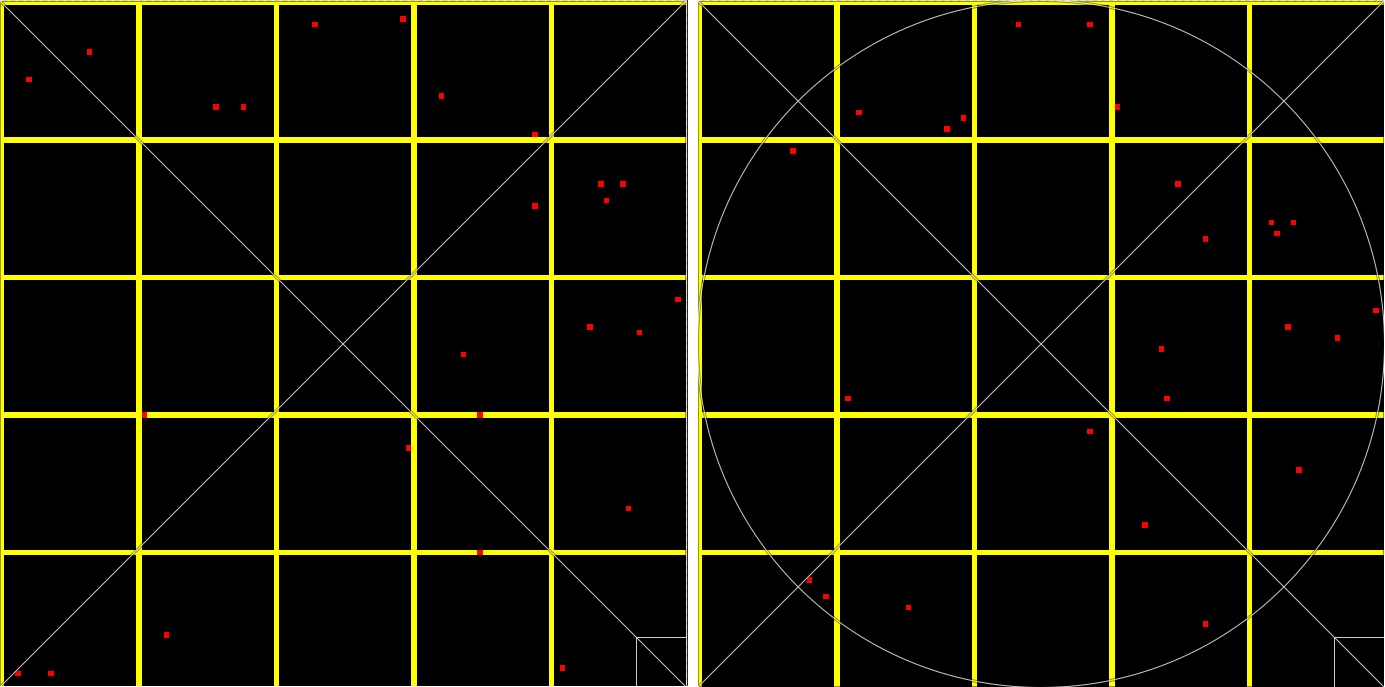
I won't go into detail here on how can we accomplish this mapping, but I'll leave a reference to Shirley and Chiu paper[4], in which they explain in details the technique. This was the paper I used to implement the mapping for my own rendering engine.

Conclusion

First part of the quest is done! Time to rest in the camp. This post was meant to be a very simple and brief introduction to the topic, with references in which you can study deeply and establish a more formal and concrete knowledge. So, get ready, because our adventure has just begun! Below is a comparison of the sampling techniques for the PFC [6] sampling technique:

Is left as a exercise to the reader the implementation of the PCF sampling technique [6], using the knowledge presented in this post as a base.

Se you in the next one! Take Care!

Bonus Content

I would strongly recommend you watch this two videos bellow, besides your reading of the reference material. Grab your coffee and dive in!

References

1 - (1978)Casting curved shadows on curved surfaces - ACM SIGGRAPH Computer Graphics, Volume 12, Issue 3 - Lance Williams

2 - (1986)Stochastic Sampling in Computer Graphics - Pixar - Robert L. Cook

3 - (1984)Distributed Ray Tracing - Lucasfilm Ltd. - Robert L. Cook, Thomas Porter, Loren Carpenter

4 - (1997)A low distortion map between disk and square - Journal of Graphics Tools - Peter Shirley, Kenneth Chiu

5 - (1987)Rendering Antialiased Shadows with Depth Maps - Pixar - William T. Reeves, David H. Salesin, Robert L. Cook

6 - (2005)Efficient Soft-Edged Shadows Using Pixel Shader Branching - NVIDIA - Yury Uralsky

7 - (1995)Principles of Digital Image Synthesis - Andrew Glassner

8 - (2007)Ray Tracing from the Ground Up - Kevin Suffern