13 minutes
Deriving the Perspective Projection Matrix
This is an updated repost of my deactivated old blog or from notes of past my studies. The date follows the original time of writing
Hi there, how your molecules doing?
Today we boldly go in one of the most important transformation in 3D Computer Graphics, namely the Perspective Projection. Doesn’t matter how deep is your knowledge of 3D graphics, whether you wrote your own raster from scratch and implemented the transformation or used it wrapped in some library with your beloved graphics API without knowing its foundations, you’ve used this matrix!
So, in this post we’re going to see how we can come up with the classic perspective projection matrix from the foundations of geometry and linear algebra. After that we’ll derive the D3D matrix and let the GL version as an exercise for the reader.
The Geometry of Projection
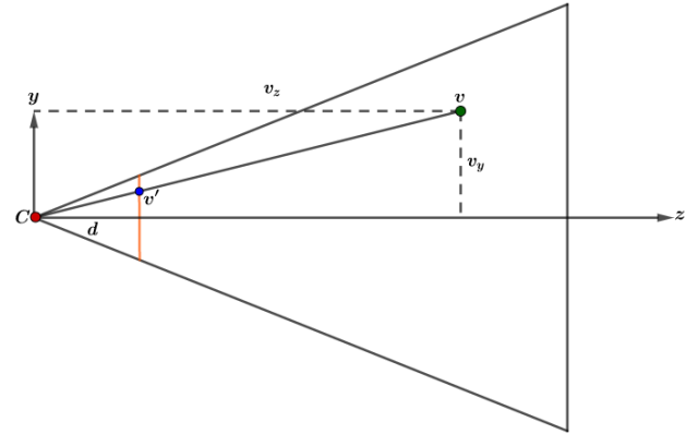
Let’s Start! The first thing I want you to pay attention is at figure 1, all the explanation I gonna give you in this next minutes is based on this picture, so active your chameleon eyes and follow me. We known for a fact that most of objects in a scene are composed of vertices (in another words: the object is a discrete group of vertices), thus we “loop” over all the vertices and transform the object as we like. This fact is great as allow us to perform parallel work in a scene, working on a lot of vertices at the same time. Therefore to project an object we need to project all its vertices, in which the order doesn’t matter as no spatial relation between vertices is needed for this operation.

Well, so how we project? It’s very simple, looking at figure 1 we can decompose \(v\) in two components \(v_z\) and \(v_y\), then by similarity of triangles we get:
\[ v'(v'_x,v'_y,v'_z) = v'(\frac{v_x}{v_z}d, \frac{v_y}{v_z}d, d) \tag{1} \]
If you’re wondering what is this \(d\) and how I got \(v'_x\) keep reading, if not skip to the next section! Well, the \(v'_x\) you can get by doing the same procedure but with the \(z\) and \(x\) axis, what about \(d\)? \(d\) is actually the distance of the projection plane (the orange line in figure 1 is a slice of the projection plane) from the center of projection \(C\), so in this case \(d\) is the bottom line segment of the smaller triangle, that’s how it end up in the formula, an interesting point to note is that d is also actually the zoom, the greater d the greater the objects appear!
Now that we known how to get \(v'\) we need a way to represent the transformation with a matrix. Enter the Homogeneous Coordinates!
Homogeneous Coordinates
When working with linear transformations (rotation,scaling,etc…) in 3D we need a 3×3 matrix, but to work with affine transformations like translation we need one more dimension, thus we work with 4×4 matrices. The perspective projection also isn’t a linear transformation, therefore we also use 4×4 matrices!
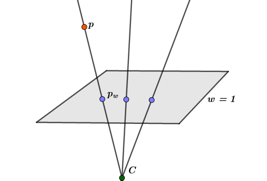
Here is when homogeneous coordinates come in hand, the notion of perspective projection and the homogeneous coordinates representation are a very good match. Take a look at figure 2:

We have a similar situation to figure 1, but now we are in 4D space (Oh yeah!) as p is a 3D vector with one more dimension w (or up if you like!), we also have \(C\), the center of projection, but here it is called point at infinity in which \(w = 0\), you’ll se why shortly. When \(w = 1\) we consider the point \(p\) to to be in homogeneous form and we call it \(p_w\), thus the name. So all the points in the direction between \(C\) and \(p\) are the same point \(p_w\) after the homogenization process, in more mathematical terms:
\[ \forall p = (x,y,z,w) \]
after the homogenization we get:
\[ p_w = (\frac{x}{w},\frac{y}{w},\frac{z}{w},1) \]
Now you can see that if \(w \rightarrow 0 \Rightarrow p \rightarrow C\), in another words if \(w\) tends to zero \(p\) tends to the center of projection or the point at infinity.
So far so good, but how this help us exactly? Well we just saw how to represent our perspective projected vertex. If you reading this
post then sure you read or heard something about the hardware z-divide, this divide is actually a homogenization if we store the \(z\) value in
the \(w\) coordinates:
- 1 -> Before the transformation we have:
\[ v = (x,y,z,1) \]
- 2 -> After the projection we have:
\[ v_p = (x,y,z,\frac{z}{d}) \]
- 3 -> And if we homogenize the vertex we get:
\[ v_w = (d\frac{x}{z},d\frac{y}{z},d,1) \]
Let’s analyze this 3 steps more carefully: The first interesting thing to note is that in 1 the vertex v is homogenized and also in 3D space while in 2 it isn’t as it is only in projective space (I believe this is the right term!), but after the homogenization in 3 the vertex return to 3D space, not in the same location though as it was projected. Another point worth mentioning is that the actual projection happens in 3 at the homogenization process, also 3 normally happens in a dedicated hardware on GPUs.
So our mission is to find a matrix \(P\) which transform a vertex \(v\) in the format 1 and return \(v_p\) in the format 2:
\[ (x,y,z,\frac{z}{d}) = (x,y,z,1)P(d) \]
Transforming to matrix form and using OpenGL column major form we get:
\[ \begin{pmatrix} x \\ y \\ z \\ \frac{z}{d} \end{pmatrix} = \begin{pmatrix} 1 & 0 & 0 & 0 \\ 0 & 1 & 0 & 0 \\ 0 & 0 & 1 & 0 \\ 0 & 0 & \frac{1}{d} & 0 \end{pmatrix} \begin{pmatrix} x \\ y \\ z \\ 1 \end{pmatrix} \]
Therefore:
\[ P(d) = \begin{pmatrix} 1 & 0 & 0 & 0 \\ 0 & 1 & 0 & 0 \\ 0 & 0 & 1 & 0 \\ 0 & 0 & \frac{1}{d} & 0 \end{pmatrix} \]
Note that: If you’re using right-hand coordinates like OpenGL does you’ll have a \(-\frac{1}{d}\) instead of a \(\frac{1}{d}\)
The matrix P we got is the perspective projection matrix [1], but the matrices we normally see in the D3D/GL docs are a lot different
from this one, so what is missing? Those matrices actually do more than projection, them transform the frustum shaped space to a
cuboid shaped one, thus making clipping easy to do. Let’s see how Direct3D does it!
From Frustum to Canonical Cuboid
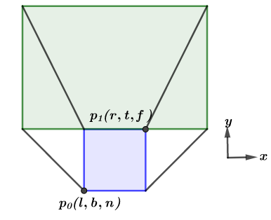
We are almost there! Now we have to find a way to convert our frustum space to a cuboid one, we have to maintain proportion in relation to size and distance between our objects, in another words we need to do a mapping between this two spaces. Look at figure 3:

Obs: \(p1\) should be \((r,t,n)\) not \((r,t,f)\), my mistake!
We have our frustum space and 2 interesting points \(p_0\) and \(p_1\), this 2 points are the extrema of the near plane, its min and max. As we are interested in placing all the points in this plane in canonical space we must map them from the projective plane (near plane) to the canonical plane. I wanna make a personal comment about this process, all the books and sources I’ve read so far (including Real-Time Rendering Third Edition) doesn’t explain in much detail this final part in which you select the near plane and assume all the points are inside it. I believe that this is intentional, to make you think and what I’m gonna present to you now is how I think about it. I gonna explain the x-axis case, you can infer the y one by symmetry. The condition a point must satisfy to be visible is that it MUST be inside the view frustum (ignoring all relation between objects, therefore ignoring hidden surface-removal algorithms for now!), this is the basic principle of the view frustum itself, thus if you draw a ray between the center of projection and the point itself it MUST intercept the near plane, otherwise the point is outside the view frustum (Draw and see for yourself!).
Now that we understand why (hopefully! If not, draw again!) we map from the near plane, it is time to do some calculations: We have all the points in the following format (forget about the z for now, think in a slice of the frustum in the x direction if you like!) :
\[\forall p(x,y) \{ p(x,y) | l < x < r \land b < y < t \}\]
and we wanna map them to the following format:
\[\forall p(x,y) \{ p(x,y) | -1 < x < 1 \land -1 < y < 1 \}\]
Let’s do some calibrations for the x case(Sorry! I mean calculations, I’m not Garrus!):
\[ - 1 < 2\frac{x - l}{r - l} - 1 < 1 \]
Therefore x and y (It’s all about symmetry my friend!) in the canonical space are:
\[x_c = 2\frac{x - l}{r - l} - 1 \land y_c = 2\frac{y - b}{t - b} - 1\]
We now work the \(z\) case, there is a point I have to make though: D3D actually map \(z\) from 0 to 1 not -1 to 1 as GL does. We now have 2 new variables \(n\) and \(f\), \(n\) is the near plane (blue one in figure3) and \(f\) the far plane (green one in figure3). Working out the math we have:
\[0 < \frac{z - n}{f - n} < 1\]
Therefore our vertex in canonical space is:
\[ v_c = (2\frac{x - l}{r - l} - 1, 2\frac{y - b}{t - b} - 1, \frac{z - n}{f - n}) \]
Now we must transform our vertex v to the canonical space equivalent v_c using a matrix transformation:
\[ v(x,y,z,1)T = v_c \]
Using matrix notation and the D3D row major notation we have (If you not comfortable with the ideia of translating operations from algebra to matrix form, well now would be a good moment to start training!) :
\[ \begin{pmatrix} 2\frac{x - l}{r - l} - 1 & 2\frac{y - b}{t - b} - 1 & \frac{z - n}{f - n} & 1 \end{pmatrix} = \begin{pmatrix} x & y & z & 1 \end{pmatrix} \begin{pmatrix} \frac{2}{r - l} & 0 & 0 & 0 \\ 0 & \frac{2}{t - b} & 0 & 0 \\ 0 & 0 & \frac{1}{f - n} & 0 \\ -\frac{r + l}{r - l} & -\frac{t + b}{t - b} & -\frac{n}{f - n} & 1 \end{pmatrix} \]
We now have our mapping matrix, which is a concatenation of both a scaling and translation transformation, think about it! Makes total sense as we scaled the frustum and then translated it:
\[ S(s)T(t) = \begin{pmatrix} \frac{2}{r - l} & 0 & 0 & 0 \\ 0 & \frac{2}{t - b} & 0 & 0 \\ 0 & 0 & \frac{1}{f - n} & 0 \\ -\frac{r + l}{r - l} & -\frac{t + b}{t - b} & -\frac{n}{f - n} & 1 \end{pmatrix} \]
If you have some familiarity with orthogonal projection you’ve probably noticed that this isn’t a perspective projection, you can see that there is not an perspective division in the transformation, therefore we must account for the perspective projection.
Let’s analyze the x case (as y is symmetrical I leave it to you!), we known that x is in the following format when using orthogonal projection:
\[ x_p = \frac{2x}{r - l} - \frac{r + l}{r - l} \]
But we also known that a perspective projected x coordinate must be scaled by d and divided by z, thus:
\[ x_p = \frac{2}{r - l}(\frac{dx}{z}) - \frac{r + l}{r - l} \]
By symmetry we also know \(y_p\):
\[y_p = \frac{2}{t - b}(\frac{dy}{z}) - \frac{t + b}{t - b}\]
Now things tend to a more engineering side than a mathematical one, as we saw early the z divide is done by the hardware, so we have to store
the \(z\) for further homogenization, but if you look at both \(x_p\) and \(y_p\) you’ll see that them already have been divided by \(z\), thus making our
math wrong, we must change that! Another point to also considere is the translation factor, which will be divided by \(z\) (this isn’t what we want
by any means!). Therefore we multiply both \(x_p\) and \(y_p\) by \(z\), and we get the coordinates in the correct format:
\( x_{p}z = \frac{2d}{r - l}x - z\frac{r + l}{r - l} \) \( y_{p}z = \frac{2d}{t - b}y - z\frac{t + b}{t - b} \)
We now look at \(z_p\), following the same parameters as before we wanna written \(z_p\) in the following way (scaling + translation) :
\[ z_{p}z = pz + q \]
But why we do this with \(z_p\) instead of just setting it to \(d\)? Well, we saw an explanation of the why our mapping from a frustum to a cuboid works (and we make sure it was right by assuming a perspective projected point), now we must remember that our vertex may be out of the frustum vision range, therefore we must map the depth of our frustum to the \([0,1]\) range, for further clipping, now note that \(z=n \rightarrow z_{p}=0 \land z=f \rightarrow z_{p}=1\).
Working the \(z = n\) case we get:
\[ q = -pn \]
And substituting \(q = -pn\) for the \(z = f\) case:
\[ p = \frac{f}{f - n} \]
Therefore:
\[ z_{p}z = \frac{f}{f - n}z -\frac{nf}{f - n} \]
I just wanna point out that the best explanation I found on the \(z_{p}z\) derivation was given by Joe Farrell in an article he wrote for Code Guru back in 2005, thus my explanation in this part was based on his article.
And finaly transforming to matrix form we have the Direct3D Perspective Projection Matrix [2], we also set our projective plane \(d = n\):
\[ P_{[0,1]} = \begin{pmatrix} \frac{2n}{r - l} & 0 & 0 & 0 \\ 0 & \frac{2n}{t - b} & 0 & 0 \\ -\frac{r + l}{r - l} & -\frac{t + b}{t - b} & \frac{f}{f - n} & 0 \\ 0 & 0 & -\frac{fn}{f - n} & 1 \end{pmatrix} \]
Working with a symmetrical projective plane we have \(|t| = |b|\) and \(|r| = |l|\), thus:
\[ P_{[0,1]} = \begin{pmatrix} \frac{2n}{r - l} & 0 & 0 & 0 \\ 0 & \frac{2n}{t - b} & 0 & 0 \\ 0 & 0 & \frac{f}{f - n} & 0 \\ 0 & 0 & -\frac{fn}{f - n} & 1 \end{pmatrix} \]
That is the matrix that the old D3DX function D3DXMatrixPerspectiveLH implements.
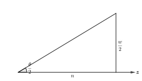
And to end with a final blast we look at the perspective projection in function of the fov, the width and the height of the projective plane! Just pay attention that instead of \(b - t\) and \(r - l\) we now use \(h\) and \(w\), that is the same for the symmetric case.

Look at the figure above, simple stuff right? Just remember your trig!
\[ tan(\frac{\theta}{2}) = \frac{w}{2n} \]
Inverting we have:
\[ \frac{1}{tan(\frac{\theta}{2})} = cot(\frac{\theta}{2}) = \frac{2n}{w} \]
Well, this result looks familiar doesn’t? Sure it does, as it is the scaling factor of the symmetrical matrix we get above, with the respective \(x\) and \(y\) versions, therefore:
\[ P_{[0,1]} = \begin{pmatrix} cot(\frac{\theta_{w}}{2})& 0 & 0 & 0 \\ 0 & cot(\frac{\theta_{h}}{2}) & 0 & 0 \\ 0 & 0 & \frac{f}{f - n} & 0 \\ 0 & 0 & -\frac{fn}{f - n} & 1 \end{pmatrix} \]
In case you just wanna work with the height fov we can use the height fov plus the aspect ratio \(\alpha\) to get the width fov:
\[ \alpha = \frac{w}{h} \]
\[ \frac{cot(\frac{\theta_{h}}{2})}{\alpha} = \frac{\frac{2n}{h}}{\frac{w}{h}} = \frac{2n}{w} \]
And we have:
\[ P_{[0,1]} = \begin{pmatrix} \frac{cot(\frac{\theta_{h}}{2})}{\alpha}& 0 & 0 & 0 \\ 0 & cot(\frac{\theta_{h}}{2}) & 0 & 0 \\ 0 & 0 & \frac{f}{f - n} & 0 \\ 0 & 0 & -\frac{fn}{f - n} & 1 \end{pmatrix} \]
This is the exactly matrix D3DXMatrixPerspectiveFovLH implements.
Well my friend our exploration is finished for today! I really expect that this post was of some assistance for you during your studies!
Any typos or mistakes just let me known and I’ll fix as fast as possible!
LIVE LONG & PROSPER
References
- [1] Foley, vam Dam, Feiner, Hughes, Computer Graphics Principles and Practice 2nd, Addison-Wesley, 1993
- [2] Akenine-Möller, Haines, Hoffman, Real-Time Rendering 3rd, CRC, 2008
2737 Words
2017-11-29 21:00 -0300