A Look at Bump Mapping Techniques - Part I: Tangent Space Theory

I - Introduction

Hello fellow life forms!

In today post, we take a look at the theory needed for understanding the famous tanget-space mapping, which is the base for most of the meso-scale rendering techniques. This post is not intended to be a in-depth mathematical treatment of tangent space, manifolds, mappings or anything like that. This is intended to lay the ground in a reasonable manner, so that when I mention Tangent Space or something related to that, you can visualize what I mean with easy.

So, let's starts by defining what we mean by Tangent Space (In a loose manner): Let \(T_s(x)\) be a real vector-space related to point \(x\) in a object. We call it a Tangent Space when such a space contais all possible tangent directions passing through \(x\). Think about a sphere \(S\), at each point \(p_s\) we can define three vectors: one alongside the horizontal, one into the horizon and other alongside the vertical. Such that, they tell how much we walk in each of those directions, if we combine these, we walk tangent to the sphere. If you are used to a little Calculus you already know this vectors are nothing more than partial derivatives \((\frac{\partial S}{\partial x}, \frac{\partial S}{\partial y}, \frac{\partial S}{\partial z})\) along \(x\), \(y\) and \(z\), respectively. We call the combination of this vectors the Gradient \(\vec{\nabla} (S)\) and it defines the tangent plane at each point \(x_s\). And yes, it is the same \(grad\) you see in ML, Optmization and Physics. Thus, mathematically we have:

\[\vec{\nabla} (x_s, y_s, z_s) . (x_s, y_s, z_s) = 0 \tag 1 \]

Well, I believe that with this little introduction you were able to, at least, get a feel for what a tanget space is! I went in a more continuous route to give the example, but in this series we gonna stick exclusive to discrete objects, i.e triangles. Continuous methods are useful, and are the right tool for other mathematical models [1], but we aren't going to look at those here! So, let's see how we can represent our Tangent Space in terms of vertices and triangles only.

II - Tangent Space

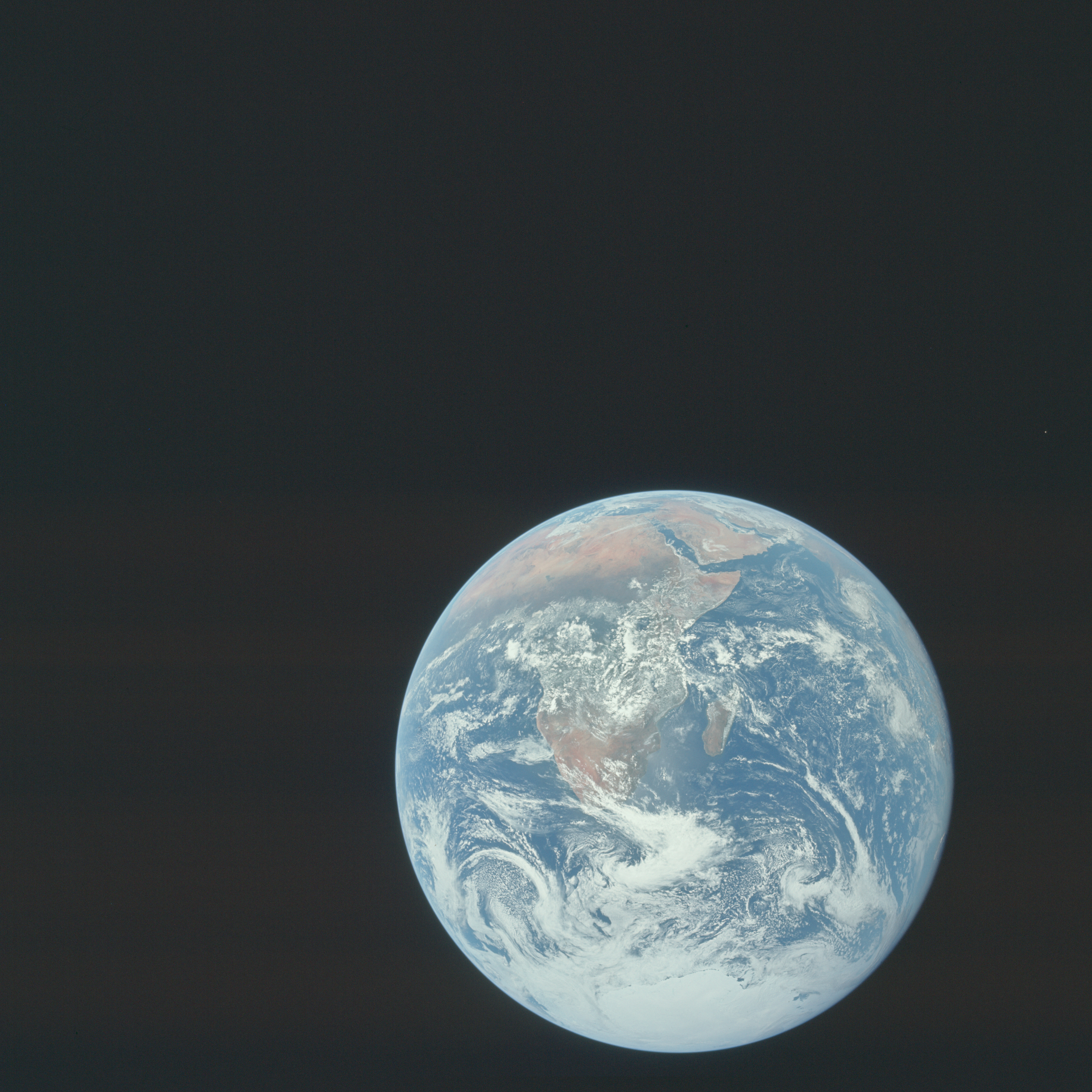
Look at figure bellow. Assume we have a discrete sphere \(S_{d}\) (in blue) and a plane \(\pi\) (in red), we can define a general vertex \(v_i\) alongside two vectors \(\vec{T}\) and \(\vec{B}\), the tangent and bitangent (the term binormal is a mistake[2]), respectively. Such that:

\[ v_i \in ( S_{d} \cap \pi) \tag 2 \]

\[ \vec{T} \land \vec{B} \in \pi \tag 3 \]

\[ \vec{T} \perp \vec{B} \tag 4 \]

\[ \vec{N} = \vec{T} \times \vec{B} \tag 5 \]

BEWARE! \(\land\) in (3) is the set notation for and, not the wedge product from Grassmann algebra.

If we were to get back to the previous example, we could make a reasonable approximation near \(v_i\), such that \(\vec{T} \approx \frac{\partial S}{\partial x}\) and \(\vec{B} \approx \frac{\partial S}{\partial y}\). Of course, the more we walk alongside these vectors the more error we get, nothing new here! Is clear we going to get error, we're approximating things since the definition of our sphere. The point to take alway is the following: The more tessellated your mesh is the smaller is the plane and so is the error. But wait! wait ... before you go nuts subdividing all your meshes to oblivion, there is something I need to mention. This is a blog focused on rendering engineering, isn't? So, I'm not just gonna say this is a implementation problem and move one, nope! As with everything in graphics/rendering this is all about visual perception, we not trying to run a precise simulation here, our goal is one such that our final render look as amazing as possible using the smallest time available! Is worth mentioning that the Bump Mapping group can be seen as a compression technique by themselves, you're mapping true geometry to heightfield representations of small areas! So don't defy its porpuse, maintain a good balance between geometry count and normal-map data resolution.

III - Calculating the Tangent and Bi-Tangent Vectors

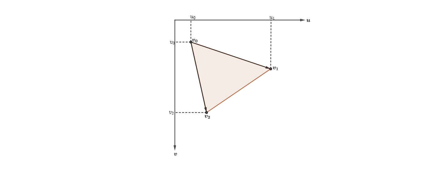
OK! Without further ado let's go down to the math! Is for this you are here, right? Looking at figure 2, above. Assume we have a generic vertex inside our triangle, let's call it \(V(u, v)\), such that:

\[ V(u, v) = \vec{v_o} + (u - u_0)\hat{u} + (v - v_0)\hat{v} \tag 6 \]

Equation (6) is nothing more than a vector inside our triangle defined in terms of \(\vec{v_0}\) as the starting point for the tail and the tip ending at some generic point (inside the triangle!) with coordiantes \((u, v)\). Let's plug \(v_1\), to see what we get:

\[ V(u_1, v_1) = \vec{v_0} + (u_1 - u_0)\hat{u} + (v_1 - v_0)\hat{v} \]

\[ V(u_1, v_1) = \vec{v_0} + (\vec{v_1} - \vec{v_0}) \]

\[ V(u_1, v_1) = \vec{v_1} \]

If you still not convinced, now would be a good moment to stop, grab piece of paper and pen an draw the geometry!

Rearranging equation (6) we get:

\[ V(u, v) - \vec{v_o} = (u - u_0)\hat{u} + (v - v_0)\hat{v} \]

\[ V(u, v) - \vec{v_o} = u\hat{u} + v\hat{v} - (u_0\hat{u} + v_0\hat{v}) \]

\[ V(u, v) - \vec{v_o} = u\hat{u} + v\hat{v} - \vec{v_0} \]

Adding \(\vec{v_0}\) on both sides, we have:

\[ V(u, v) = u\hat{u} + v\hat{v} \tag 7\]

Applying (7) to both \(\vec{v_1}\) and \(\vec{v_2}\):

\[ V_1(u_1, v_1) = \vec{v_1} = u_1\hat{u} + v_1\hat{v} \\ V_2(u_2, v_2) = \vec{v2} = u_2\hat{u} + v_2\hat{v} \tag 8\]

Wait a minute ... We now have a 2x2 system of equations:

\[ \begin{pmatrix} V_1 \\ V_2 \end{pmatrix} = \begin{pmatrix} u_1 & v_1 \\ u_2 & v_2 \end{pmatrix} \begin{pmatrix} \hat{u} \\ \hat{v}\end{pmatrix} \tag 9 \]

Let's see what we know about it! We already know the values of both \({V_1}\) and \({V_2}\). We also know \(u_1\), \(u_2\), \(v_1\) and \(v_2\), they are given! So... we ended up with? Yeah! You guessed it! It is \(\hat{u}\) and \(\hat{v}\). Solving it using Crame's Rule, we get:

\[ \begin{pmatrix} \hat{u} \\ \hat{v} \end{pmatrix} = \frac{1}{u_1v_2 - u_2v_1}\begin{pmatrix} v_2 & -v_1 \\ -u_2 & u_1 \end{pmatrix} \begin{pmatrix} V_1 \\ V_2 \end{pmatrix} \tag{10} \]

So, there you go! We now have two vectors \(\hat{u}\) and \(\hat{v}\) that follow all the constraints we established in section II. We are done then, right? Well... Not exactly, you may have noticed that in any moment I mentioned the vectors \(\vec{T}\) and \(\vec{B}\). So, what's up with that? Well, as it turns out \(\hat{u}\) and \(\hat{v}\) do not represent the tangent vectors for a vertex in tanget-space, but instead they represent the tangent vectors for a triangle in texture-space! Let's see how we can fix that.

IV - Practical Considerations

-> First, we must go from a triangle to a vertex: To do so we must first analyse a vertex and what is adjacent to it. If you look at a peak vertex you can see that it represents (approximately) a region in which we should have a smooth surface. Thus, to correctly represent the information present on this point we must average the information of all \(k\) triangles that share this vertex \(v_i\):

\[ v_{i}' = \frac{\sum_{i=0}^{k}v_i}{||{\sum_{i=0}^{k}v_i}||} \tag{11} \]

-> Second, after the previous process of smoothing the vertices and then linearly interpolating it for pixel shader consumption, we lose propriety (4) from section II. Therefore, we should also use the Gram–Schmidt process to maintain our vectors perpendicular to each other!

Finally! We now have two vectors \(\vec{T}\) and \(\vec{B}\), such that all properties from section II are preserved and we can safely use them to transform between world/object and tangent spaces for our needed calculations. But this is a topic for the next post! See you there, bye!

Live long and prosper!!!

References

1 - (1978)Simulation of Wrinkled Surfaces - Jim Blinn - Association for Computing Machinery, Inc.

2 - (2011)Mathematics for 3D Game Programming and Computer Graphics, Third Edition - Eric Lengyel - Cengage Learning PTR