Math & Games: Three Revolutionary Equations

Hi folks! How are your molecules doing?

In December 2025 I had the pleasure of speaking at the PlayMinas Intergame Summit, the first scientific congress of the games industry in Brazil, right here in Belo Horizonte. The talk was in Portuguese, Matemática & Games: 3 Equações Revolucionárias, and the recording is on PlayMinas’ YouTube channel, under the session’s title in the program, Matemática da Luz. This post is the English version, slides included.

The idea was simple: take three equations that most of us met in school and show how each one became a revolution in games, first in software and then, eventually, in silicon. No magic, just math (and a few decades of very clever engineering)!

The title slide of the talk — Matemática & Games: 3 Equações Revolucionárias – PlayMinas Intergame Summit, Belo Horizonte, December 2025.

Equation I: The Dot Product

Our first guest is the humble dot product. It has two faces, and both matter:

\vec{a} \cdot \vec{b} = a_1 b_1 + a_2 b_2 + \dots + a_n b_n = |\vec{a}|\,|\vec{b}| \cos\theta

The algebraic form is what the hardware computes: multiplies and adds. The angular form is what we mean: how aligned two directions are.

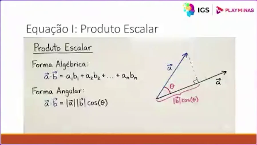
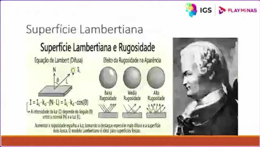
Slide: the dot product — Equation I: the dot product, in its algebraic and angular forms.

That second meaning is exactly what Lambert needed. For a perfectly matte (Lambertian) surface, the reflected intensity only depends on the angle between the surface normal $\hat{N}$ and the direction to the light $\hat{L}$ :

I = I_L\, k_d\, (\hat{N} \cdot \hat{L}) = I_L\, k_d \cos\theta

Rough, matte surfaces scatter light in every direction, which is why this simple model works so well for them.

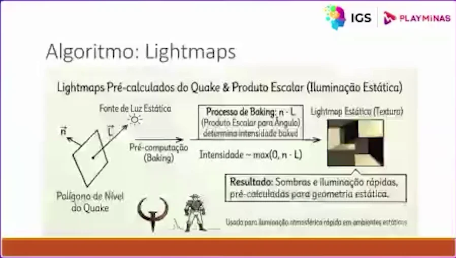
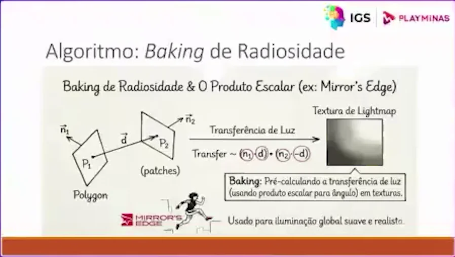
Slide: Lambertian surfaces — Lambertian surfaces: the diffuse term is a dot product, and roughness spreads the light.

Now, computing that for every pixel, every frame, was way too expensive in the 90s. Quake’s answer was to do it once: bake the static lighting into textures, the famous lightmaps, with an intensity proportional to $\max(0, \hat{n} \cdot \hat{L})$ , and simply read it back at runtime. Fast lights and shadows for static geometry, paid for at build time.

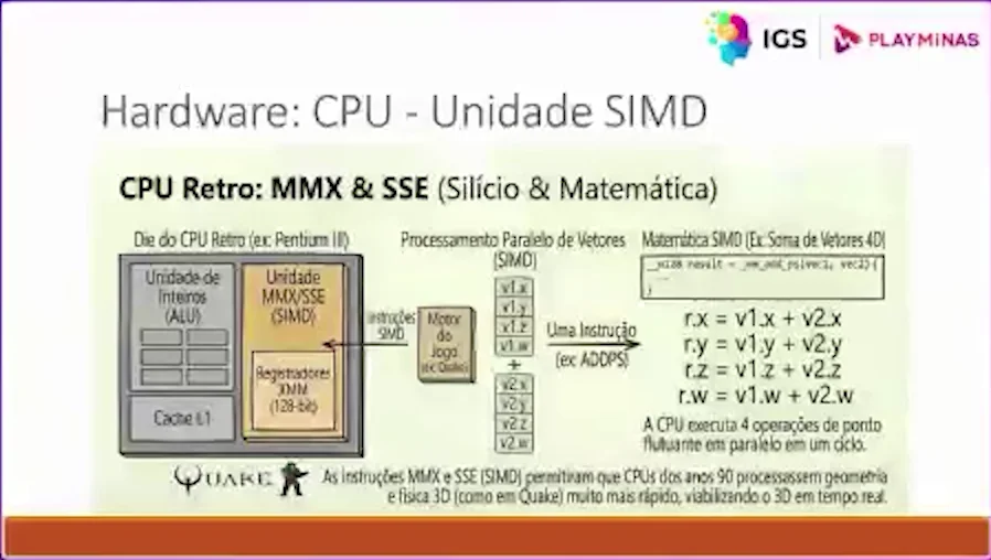
Slide: Quake’s lightmaps — Quake’s precomputed lightmaps: the dot product, baked into a texture.

And since games do a lot of dot products, CPUs eventually grew hardware for them. SIMD extensions like MMX and SSE let a single instruction (e.g. ADDPS) operate on four floats at once, in 128-bit XMM registers. Silicon, meet math.

Slide: SIMD on the CPU — CPU SIMD: one instruction, four floating-point operations.

Equation II: The Rendering Equation

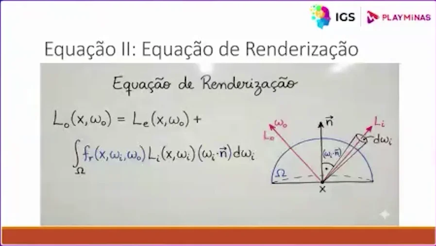
The second equation is the one at the bottom of every page of this blog, Kajiya’s rendering equation (1986):

L_o(\mathbf{x},\omega_o) = L_e(\mathbf{x},\omega_o) + \int_{\Omega} f_r(\mathbf{x},\omega_i,\omega_o)\, L_i(\mathbf{x},\omega_i)\, (\omega_i \cdot \hat{\mathbf{n}})\, d\omega_i

The light leaving a point is the light it emits plus all the light arriving from the hemisphere above it, weighted by the BRDF and, look who’s back, a dot product. It describes global illumination completely, which is exactly why it is so hard to solve.

Slide: the rendering equation — Equation II: the rendering equation.

For years the practical answer was, again, baking. Radiosity splits the scene into patches and computes how much light flows between each pair, a transfer that depends on how much the two patches face each other, $(\hat{n}_1 \cdot \hat{d})(\hat{n}_2 \cdot -\hat{d})$ , and stores the result in lightmaps. Mirror’s Edge is a beautiful example of what that soft, baked global illumination can look like.

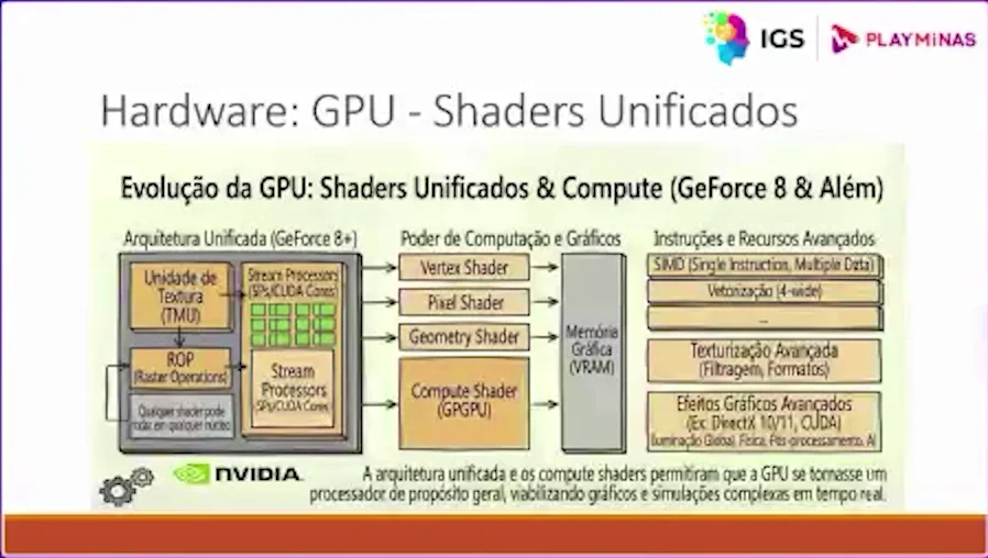
Slide: radiosity baking — Radiosity baking: light transfer between patches, precomputed into lightmaps.

What changed the game was the GPU becoming a general-purpose processor. With unified shaders (GeForce 8 and beyond), the same stream processors run vertex, pixel, geometry and compute work, and compute shaders opened the door to solving much more of the rendering equation every frame. That is the road that led to real-time path tracing in games like Cyberpunk 2077.

Slide: unified shaders — Unified shaders and compute: the GPU as a general-purpose processor.

Equation III: The Quadratic Equation

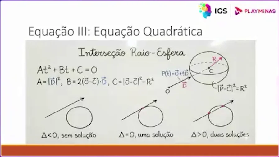
To trace a ray we need to know what it hits, and our third equation answers that. A ray is $P(t) = \vec{O} + t\vec{D}$ , and a sphere is every point with $|P - \vec{C}|^2 = R^2$ . Plug one into the other and you get the good old quadratic:

A t^2 + B t + C = 0, \quad A = |\vec{D}|^2,\quad B = 2(\vec{O} - \vec{C}) \cdot \vec{D},\quad C = |\vec{O} - \vec{C}|^2 - R^2

The discriminant $\Delta = B^2 - 4AC$ tells the whole story: $\Delta < 0$ , the ray misses; $\Delta = 0$ , it grazes the sphere; $\Delta > 0$ , it enters and leaves.

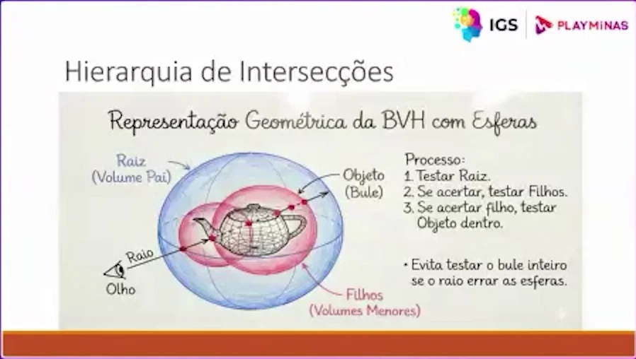
Slide: ray–sphere intersection — Equation III: ray–sphere intersection is a quadratic equation.

Testing every ray against every triangle would take forever, so we wrap the scene in a hierarchy of bounding volumes (a BVH): test the root first; only if the ray hits it, test the children; only then test the object inside. If the ray misses the big sphere, we never touch the teapot at all.

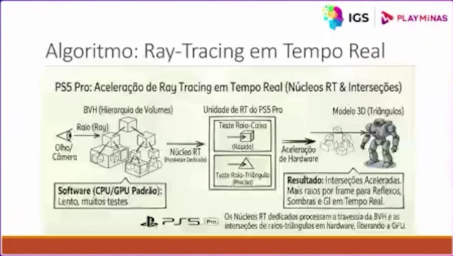
Slide: bounding volume hierarchy — A bounding volume hierarchy: skip the teapot unless the ray hits its bounds.

And here is the final plot twist: these tests now live in silicon. Dedicated ray tracing units, like the ones in the PS5 Pro, traverse the BVH and run the ray–box and ray–triangle tests in hardware, freeing the shader cores for everything else. That is what makes reflections, shadows and global illumination possible in real time, in games like Ratchet & Clank: Rift Apart.

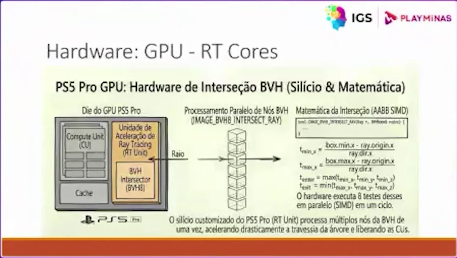
Slide: real-time ray tracing — Real-time ray tracing: BVH traversal and intersections in dedicated hardware.

Zoom into one of those units and you find our math again. A single instruction, IMAGE_BVH8_INTERSECT_RAY, tests a ray against eight boxes of a BVH node at once with the slab method:

t_{min} = \frac{box_{min} - ray_{origin}}{ray_{dir}}, \quad t_{max} = \frac{box_{max} - ray_{origin}}{ray_{dir}}

t_{enter} = \max(t_{min,x}, t_{min,y}, t_{min,z}), \quad t_{exit} = \min(t_{max,x}, t_{max,y}, t_{max,z})

The ray hits the box when $t_{enter} \le t_{exit}$ . Eight of those per instruction, in parallel. SIMD again!

Slide: RT cores — Inside the RT unit: eight ray–box slab tests per instruction.

Conclusion

Three equations: a dot product, an integral and a quadratic. The first lit Quake, the second drove decades of research in global illumination, and the third ended up as an instruction in a GPU’s ISA. Every time the math got too expensive, we first baked it, then built hardware for it.

Thanks again to the PlayMinas team for the invitation, and to everyone who came to Sala 3!

Live long and prosper!